(This piece is written in part by AI, in particular Fable 5. My original piece, in my voice, is here)
Summary of claims. (1) The wage is a bundled institution performing four functions — pricing labor, distributing output, transmitting demand information, and structuring social life — whose load-bearing assumption is that production needs nearly everyone. (2) Automation erodes that assumption cohort by cohort and place by place; the evidence is real but entangled with endogenous “absorption” institutions, and the identification problem is stated. (3) Chaining distribution to labor-market participation produces two structural failures: the economy has no sufficiency signal, because the participation margin never faces an honest market test; and it systematically violates production efficiency, because jobs are scored as benefits when they are costs. (4) In the automation limit, factor income converges to rents on non-reproducible factors; the only politically stable configuration disperses ownership of that base; and prices must be retained, because they are the economy’s demand-elicitation mechanism, not a computation a planner can replicate. (5) The implied design is three mechanisms, launched together: a universal cash floor; claims on the scarce base — a land-value tax accumulating into a buy-side sovereign equity fund; and a VAT surcharge that carries the floor’s funding while the base matures — incidence-equivalent to a flat consumption tax plus demogrant and, taken seriously, also a one-time levy on existing wealth recycled as a perpetual flow: a crude, single-shot rehearsal of the destination, with a hard ceiling, a capitalization pressure the co-launched land tax exists to intercept, and tractable stabilization plumbing. (6) Its macroeconomics are two separable channels: a one-off price-level step during the ramp, and a demand effect that is approximately neutral in a Nordic wealth distribution and mildly negative in an American one — inflationary in the price-level sense, weakly disinflationary in the demand sense, but dependent on wealth levy perception.
The wage as a bundled institution
A wage does four jobs at once. It is a price, allocating people across uses and disciplining production costs. It is a claim: for nearly all households, selling labor is the only mechanism by which the economy owes them output — pensions are deferred wages, insurance benefits are conditioned on wages lost, and capital income is held by people who were never waiting on the channel. It is a signal: spent wages are the demand half of the price system, and a person with no purchasing power is a sensor the market cannot read, which makes distribution a question of informational bandwidth and not only of equity. And it is a bundle of non-pecuniary goods — time structure, status, contact, purpose — whose loss damages people even under full income replacement, a result stable since the Marienthal studies.[^1]
One instrument, four functions. The arrangement works exactly as long as production needs nearly everyone’s labor, so that labor can serve as the universal claim. The interesting question about automation is not “will there be jobs” — job creation and displacement coexist trivially — but which of the four functions survives the erosion of that universality, and what replaces the ones that don’t.
Evidence, with the identification problem
Two headline statistics get cited as if they settled the question, and neither can. The unemployment rate conditions on searching for work, so everyone an absorption institution has reclassified — retired, enrolled, assessed as unfit — simply vanishes from it. Aggregate participation counts them, but as one number moved by demographics, schooling norms, and pension rules all at once, it can drift for half a century without disclosing which force did the work. The series worth reading sit underneath both, and before listing them, the honest methodological note.
The hypothesis doing organizing work in this essay is that several large institutions — retirement, extended education, disability — function partly as absorption mechanisms: endogenous responses that relabel weak labor demand as a life stage, a training period, or a health state. This hypothesis is observationally close to the benign reading in which those institutions reflect demographics and rising returns to schooling. Both are partly true; they are overdetermined institutions. Pensions emerged from labor movements and coalition politics as much as labor-demand arithmetic, and for most of the twentieth century education expansion tracked genuinely rising skill demand — the Goldin–Katz race, which education was mostly winning.[^2] The absorption reading fits the margins (credential inflation, lengthening duration, parking of the young), not the core. I cannot separate the hypotheses with aggregate data, so I will state the margins where they diverge and the observations that would falsify my reading, below.
The dials:
- Prime-age men. US participation for men 25–54 fell from 98% in the mid-1950s to about 89%; among those with high school or less, from over 96% to 83%. Disability insurance absorbs little of it — SSDI receipt rose roughly 1.5 points over a period in which participation fell 8.4.[^3] Note that this cuts against a pure absorption story: this is the unpatched failure mode, exit recorded by no program. Supply-side explanations (spousal income, transfers, caregiving) account for little of the trend.[^4]
- Factor shares. The global labor income share has drifted down since the 1980s — roughly five points to its mid-2000s trough, 53% to 52.4% in the last decade alone — and the US labor share stands at its lowest since the Great Depression.[^5][^6] The strongest critique: Rognlie showed that the entire postwar rise in the net capital share across the large developed economies comes from housing; ex-housing, capital’s net share has gone roughly nowhere.[^7] Read one way this deflates “automation is eating labor’s share.” Read the other way it is the single most important stylized fact below: returns are already concentrating into the non-reproducible factor. Hold it for the limit section.
- AI and the entry margin. Since late 2022, employment for workers aged 22–25 in the most AI-exposed occupations has fallen 13–16% relative to other groups, while experienced workers in the same occupations and young workers in unexposed occupations are flat or growing. This is a working paper and should be priced as one, but it is not naive: the result survives excluding technology firms and remote-amenable occupations; the exposure taxonomy has no predictive power for young workers’ outcomes pre-LLM, including through the COVID shock; it replicates in public CPS data; and the declines concentrate where adoption automates tasks rather than augments workers.[^8] Recent-graduate unemployment now exceeds the overall rate for the first time in the modern record; the gap is small.[^9] Early, revisable — but the pattern is precisely where a substitution story predicts first incidence: the entry rungs.
- The improvised second pipe. US government transfers are 18% of personal income, up from 8% in 1970; a majority of counties now draw a quarter or more of income from transfers, against fewer than 1% of counties fifty years ago.[^10] Composition honesty: most of the growth is Social Security and Medicare — aging plus healthcare inflation — so this is not, by itself, evidence that the wage channel failed. What it establishes is narrower and sufficient: a non-wage distribution system already operates at the scale of a sixth of all personal income, assembled categorically, one emergency at a time, with screening costs, participation cliffs, and no design.
Falsification. The reading above is wrong if, over the next five years: prime-age participation rises broadly through AI diffusion; the entry-level employment gap closes as the rate cycle normalizes; bottom-decile wages keep gaining on the median without policy force; the ex-housing labor share turns durably upward; or the canaries result washes out under revision. In that world, the design below was built early, and its cost was a modest progressive consumption tax with a demogrant and an automatic stabilizer attached. The asymmetric loss sits on the other branch.
Failure one: no sufficiency signal
Keynes’s 1930 extrapolation — productivity gains partly cashed out as time — worked for a century: annual hours roughly halved between 1870 and the 1970s. Then the paths split; continental Europe kept converting some gains into time while US hours flatlined (taxes, unions, preferences — pick your school), and much of the leisure that did arrive came in blocks at the edges of life, retirement and extended education, rather than as shorter weeks in the middle.[^11]
The structural reason the mechanism cannot complete is that in a wage-distribution economy, “we need less labor” has no way to arrive as good news; it can only arrive as someone’s zero. So the institutional stack is built — rationally, locally — to suppress the signal: employment mandates, payrolls as the success metric of stimulus, jobs as the unit of political accounting. The panel has gauges for inflation, unemployment, and growth, and no gauge for enough.
The standard reply is that “enough” is undefined because wants are unbounded. Perhaps. But the claim is never tested, and here is the precise sense in which the test is rigged. The competitive benchmark — wages track marginal product — is a statement about the wage level; the failure is at the participation margin. A worker whose entire claim on subsistence routes through employment has a reservation wage pinned near subsistence rather than at the social opportunity cost of their time. Jobs whose output is worth less than any dignified valuation of that time get created and staffed anyway, and the fact of their staffing is then cited as revealed preference that the work was worth doing. Monopsony evidence reinforces the point at the wage level too,[^12] but the argument does not depend on it: run an auction in which one side cannot walk away, and the hammer price carries no information about whether the lot was worth selling.
Failure two: production inefficiency by design
In cost–benefit analysis, labor is an input: a cost, the valuable time a project consumes. In a wage-distribution economy the sign flips and jobs are scored as benefits — by politicians, development agencies, planning processes, bailout metrics. The exception is real and bounded: where the shadow wage is below the market wage (depressed regions, deep slumps), job creation has genuine transfer value. The error is letting that emergency logic set the steady state.
The inversion moves real resources. Land and infrastructure concentrate where the remaining labor-intensive, face-to-face work lives, because proximity to a job is the price of holding a claim; some of that is genuine agglomeration productivity, some is claim-chasing, and current accounting cannot distinguish them. Capital tilts toward employment-visible projects. And the bottom of the service sector operates at a scale set by desperation pricing: a business model that clears only because its workers lack an outside option is receiving an input subsidy, paid in kind by its own workforce. Sectors thus exert gravitational pull on land, talent, and policy in proportion to the claims they distribute rather than the output they produce — a market distortion by the textbook definition, unnamed because the distorting institution is the labor market itself. The system functions as a welfare state run through the side door of payroll, with the deadweight billed to everyone and itemized to no one.
The limit case
Take the endpoint seriously as a model: production needs almost no one, machines reproduce machines, the marginal cost of reproducible goods falls toward energy and materials. Labor income goes to zero share; returns on reproducible capital get competed toward commodity margins. What remains is income to non-reproducible factors: land and location, resource and energy flows, spectrum, the atmosphere’s absorptive capacity, and legal artifacts — patents, licenses, market position. In the limit, all income is rent, and the ownership question is the only question.
Only the dispersed-ownership configuration of that endpoint is stable. Concentrated rentier ownership with universal suffrage does not sit still: it resolves into redistribution or into the end of the franchise, and history offers exits in both directions, none gentle. A universal claim on the scarce base — a dividend — is the arrangement in which markets, democracy, and full automation survive contact with each other. And per Rognlie, the convergence is not prospective: the developed world’s net capital-share rise has already been, in its entirety, a land story.[^7]
What must survive in any configuration is the price system, and the reason is worth stating before its AI-flavored challenge arrives. Prices are not a computation a sufficiently large planner replicates; they are a measurement — the only incentive-compatible instrument that elicits preferences at scale, by making people choose under budget constraints. An economy that stops asking people, each holding purchasing power they may point anywhere, has not automated demand; it has amputated it. The dividend is the sensor grid as much as it is the equity instrument.
Non-solutions, briefly
Robot taxes and protection violate production efficiency — Diamond–Mirrlees says don’t tax intermediate inputs; tax rents and consumption and leave the production side undistorted — while slowing the abundance that funds everything else.[^13] Scaling means-tested categories compounds effective-marginal-tax-rate cliffs and screening costs, and requires a new deservingness category per displaced cohort; the UK’s binary “can/cannot work” assessment is the live cautionary case of classification incentives doing the absorbing. “Everything gets cheap” fails on composition: the automatable half of the basket deflates while the scarce half — housing — absorbs the gains, which is Rognlie’s fact operating at the level of household budgets. A job guarantee takes the non-pecuniary bundle seriously but preserves the form by having the state invent the content: the participation-margin test stays rigged and the missing gauge stays missing.
The design: three mechanisms
Mechanism one: the floor. A universal, individual, unconditional cash payment. Universality is mechanism design, not generosity: a zero marginal withdrawal rate (earnings always add — no EMTR spikes anywhere in the distribution), no screening or ordeal costs, no classification incentives of the kind currently filling incapacity rolls, and political durability — a program every citizen receives is one no government quietly cuts, as Alaska has demonstrated since 1982. A floor, not a livelihood, at first.
Mechanism two: the base. The funding source decides whether the system survives the trend it is built for, and the limit case dictates it: claims on non-reproducibles, plus equity in the machines.
Rents first, and from the first day. Land value capture is the textbook non-distorting tax — supply elasticity zero, the base immobile, and (per the Henry George theorem in its weak form) large enough to matter[^14] — and it is the base that grows as automation concentrates returns into scarce factors, which the Rognlie decomposition says has been happening for decades. It launches with the dividend rather than after it, for a reason the bridge’s own charts supply below; its incidence and revenue are left unmodeled in this essay because they depend on rate, assessment, and exemption choices that sit downstream of the modeling here. The cadastral infrastructure mostly exists; Denmark has assessed land separately for a century. Then spectrum, resource royalties, congestion, carbon.
Equity second, and precision matters because there is an honest instrument and a seductive one. The seductive instrument is the share levy — tax firms in newly issued stock, Meidner-style. Sweden ran the experiment’s neighborhood once; the wage-earner funds were politically annihilated within seven years, and the rolling dilution of listed firms was the firestorm at least as much as the collective governance.[^15] The honest instrument is buy-side: rent revenues and bridge surpluses accumulate in a sovereign fund that purchases the capital stock at market prices, Norway-style — individually attributed claims, levy-free acquisition. The buy-side route also answers an objection nothing else in the design reaches: a small open economy cannot tax the rents of a foreign model company — corporate tax stops at the border and the IP books elsewhere — but it can own them. Norway’s fund holds on average roughly 1.5% of every listed company on earth.[^16] What sovereignty cannot reach, a brokerage account can; the dividend then grows with the machines wherever they are incorporated.
Mechanism three: the bridge. Fund accumulation takes a decade-plus and land assessment ramps over years; the floor needs full revenue from the first month, and the one base that delivers it immediately is consumption: a uniform VAT surcharge financing the flat dividend.

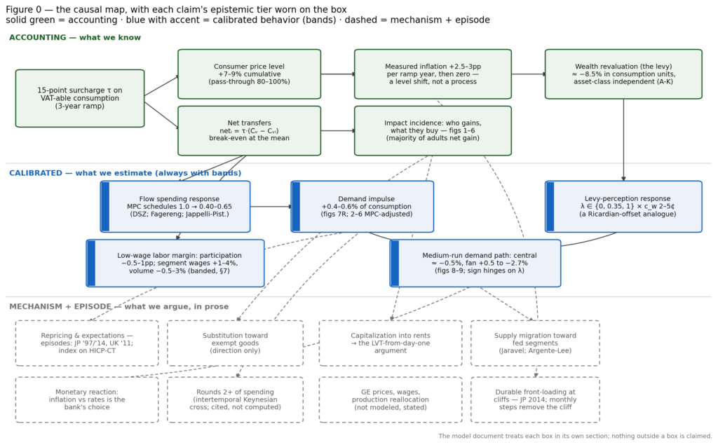
Figure 0 — the map of what follows. Every causal claim in the bridge analysis, with its epistemic tier worn on the box: solid green is accounting (identities and mechanical arithmetic; data quality is the only error source), blue with the accent bar is calibrated behavior (named parameters, always shown with bands), dashed gray is mechanism-plus-episode (argued in prose, anchored to a cited natural experiment, never drawn).
The mechanics are friendlier than VAT’s reputation. With surcharge rate τ on VAT-able consumption and a balanced budget, each adult pays τ·Cᵢ and receives τ·C̄, so the net transfer is
netᵢ = τ·(C̄ − Cᵢ) —
linear in consumption, progressive over consumption by construction, with break-even at the mean; since consumption is right-skewed, a majority of adults are mechanical net recipients. Figure 1 puts real numbers on it, from Finland’s 2022 Household Budget Survey — the most recent Nordic consumption-by-quintile survey in existence, Sweden’s having been discontinued after 2012 with the next wave only now in the field.[^22] A 15-point surcharge on the existing VAT base funds a dividend of €193 per adult per month, each child adding a 30% share; the net runs from +€77 a month per adult share for the bottom quintile (+5.9% of its budget) to −€88 for the top (−3.1%), with the middle quintile sitting within €5 of break-even.

Figure 1 — tier: accounting. Net monthly effect (dividend received minus extra VAT paid) of a 15-point surcharge funding a flat per-adult dividend (each adult one share, each child 0.3), Finland 2022, per adult share. The relation is exactly netᵢ = τ·(C̄ᵥ − Cᵥᵢ) per share on VAT-able consumption, which runs from 59% of the bottom quintile’s budget to roughly two-thirds in the upper quintiles — lowest at the bottom, because the largest exempt item, rent, weighs heaviest in poor households’ budgets, which makes the surcharge marginally more progressive than a tax on total consumption would be. Quintile means compress the tails: individual households extend well past these five points in both directions, so the figure understates the spread of net positions, not the mechanism. No behavioral assumption enters; the only judgment inputs are the per-category VAT-ability.
A second property follows from uniformity: a flat surcharge leaves relative prices unchanged, so the first-order reallocation of demand across goods is a pure income effect of the redistribution — no substitution effects to model, and an argument for keeping the surcharge uniform rather than importing the exemption lattice of existing VATs (the theory case for uniformity is Atkinson–Stiglitz; the EU’s own accounting makes the practical case, with revenue forgone to reduced rates and exemptions running at six times the revenue lost to non-compliance[^24]). Figure 2 runs the income effect through the data at the second COICOP level: quintile market shares for each line of the family budget from the same Finnish survey, income elasticities computed per quintile from the Working model — η = 1 + β/w, with β from USDA’s 144-country demand system, so that food’s elasticity falls from 0.44 in the bottom quintile to 0.30 in the top without anyone assuming it[^23] — and each quintile’s budget shock scaled by its marginal propensity to consume out of a permanent flow, with the MPC=1 benchmark left visible as a ghost outline on every bar.[^27] The MPC gradient matters more than it sounds: recipients spend roughly all of a permanent transfer while payers finance much of theirs from saving, so the adjusted bars no longer sum to zero — their sum is the aggregate demand impulse, +0.4% of charted budget in Finland — and several knife-edge categories flip sign outright once the top’s withdrawal halves, vehicle operation among them. Three readings. First, the scale: the largest single reallocation in the basket is about €5 per adult-share month, on budgets averaging €2,051 — a transfer worth three to eight percent of budgets moves purchasing power without much reshaping relative demand. Second, the impact period is nearly all green: at launch, this policy is almost pure demand addition, the withdrawals arriving later and smaller. Third, where the largest bar sits: actual rents, +€4.92 a month. Renters are concentrated precisely where the net transfers land, so the figure shows the capitalization leak (taken up below) from the demand side, before a landlord has repriced anything — the empirical reason land taxation starts on day one rather than on layer two’s schedule.


Figure 2 — tier: accounting incidence × calibrated behavior (η, MPC); the MPC=1 first-order benchmark is the ghost outline. Impact-period changes in spending by COICOP second-level category, euros per adult share per month (percentage change in parentheses): Δ€g = Δ%g·C̄g with Δ%g = Σq θqg·ηgq·(mpc_q·netq/Cq). Elasticity fidelity is at the parent-group level — subcategories inherit their group’s quintile-specific η, with the food system split via the stage-two parameters — while the incidence θ is each line’s own. Caveats: cross-country β applied within-country (a use the source itself endorses); education omitted, since a 0.3% budget share makes β/w numerically meaningless; imputed and owner-occupied housing omitted, since nothing is transacted there; impact-period only — the rent bar is the demand impulse, not the post-capitalization equilibrium: landlords are the other claimant on that €5.
What no category bar can show is the margin inside it: every line of Figure 2 spans a quality ladder — used cars and new ones, discount groceries and delicacies, studio rentals and penthouses — and a transfer from the top of the distribution to the bottom should walk demand down each ladder even where the category total barely moves. Expenditure data records price times quantity fused, so quality cannot be separated from volume without quantities (the unit-value method of Deaton, which needs the survey microdata). But the first-order geometry is already in the model: each category’s change decomposes by quintile, and quintiles occupy rungs. Figure 3 opens the ten largest movers. Vehicle purchases are the one red bar left standing at impact: the top two quintiles withdraw new-car money faster than the bottom three add used-car money, for a net of −€0.5 that conceals gross tier rotation several times its size. Rents are the mirror case: the +€5 is almost entirely bottom-quintile money, concentrated on the cheap end of the housing stock, which localizes the capitalization pressure too. The mapping from quintile to rung is imperfect — the rich shop at discounters too — but the supply side takes it seriously: product entry follows growing demand segments, and recessions run the same film in reverse as households trade down within categories.[^25] If anything the composition shift is the larger long-run story: variety and quality competition migrating toward the segments the dividend feeds.


Figure 3 — tier: same hybrid as Figure 2. The ten largest impact-period movers, decomposed by quintile: green segments are demand added by the gaining quintiles (Q1–Q3), red is demand withdrawn by the paying quintiles (Q4–Q5); the solid diamond marks the MPC-adjusted net, the hollow diamond the MPC=1 net. Where quality tiers track buyers, the gross flows are the within-category composition shift — the same category growing at its cheap end while shrinking at its expensive end.
The rent result invites a question the design should answer before going further: if rents are where the money lands, why not pull rents inside the VAT and tax them there? Because two-thirds of households consume housing services from a dwelling they own, and imputed rent cannot be taxed — nothing is transacted. Taxing actual rents while imputed rent walks free is not a tax on housing; it is a tax on renting, levied on the tenure group that is two-thirds of the bottom decile and a tenth of the top, and it would partially undo the progressivity that Figure 1’s caption credits to the exemption. The steelman — in supply-inelastic markets a rent tax falls largely on landlords — fails three ways: it misses the owner-occupied half of the land base entirely, it taxes the structure along with the land (and new construction already carries VAT, so rental housing alone would be taxed twice), and its incidence flips onto tenants exactly where supply is elastic. Notice instead what the standard design already does: new construction is taxed — prepaying the VAT on that dwelling’s entire future stream of housing services, tenure-neutrally — and the subsequent flow is exempt. What escapes the consumption tax is therefore precisely the existing stock: land plus old structures. The hole in the VAT is shaped exactly like the scarce-rent base, and the instrument shaped exactly like the hole is the land-value tax — which reaches land under every tenure, exempts structures, and cannot be shifted. The bridge structurally cannot tax the destination’s base; that is the formal version of why the bridge is not the destination.
The same exercise runs on American data — the Consumer Expenditure Survey’s 2024 deciles — with two translations: the United States has no VAT, so the flags describe an EU-style base being introduced, and the survey reports unequivalized consumer units, so everything is converted to payment units — one share per adult, 0.3 per child — using the table’s own household-composition rows.[^26] The shape survives the Atlantic, and deciles restore the tails the Finnish quintiles compressed (Figure 4): fifteen points on that base fund about $249 per adult per month, seven deciles gain, break-even falls between the seventh and eighth, and the top decile pays $173 a month net per adult share (−3.9% of its budget). The demand shifts (Figure 5) replicate the headline: the largest single mover is again rented dwellings, +$3.36 a month — the rent result is not a Nordic artifact. And because the American table splits vehicle purchases by tier, the quality-ladder conjecture of Figure 3 becomes a measurement: with the MPC gradient applied, new cars fall (−$0.39, against a first-order ghost of −$1.23) while used cars rise (+$0.38, flipped from a first-order −$0.05) — the walk down the ladder visible as opposite signs on the two ends of the same showroom. Two American inversions earn a sentence each. Out-of-pocket health and vehicle insurance rise with the dividend (+$1.08, +$0.53): what the Nordic state provides as a service, the American bottom deciles buy as a necessity, so handing them cash buys coverage — and health insurance is the basket’s biggest churner, gross inflow from the gaining deciles running several times the top-side trim. And the payer-concentrated discretionary margin — fees and admissions, vacation lodging — shrinks only modestly at impact (−$0.20, −$0.13), its larger contraction arriving with the wealth channel below.

Figure 4 — tier: accounting. Net monthly effect per adult share (each adult one share, each child 0.3 — the flat payment rule) of a 15-point consumption tax on an EU-style VAT base funding the dividend, by pretax-income decile, Consumer Expenditure Survey 2024. The dots do not fall strictly in income order through the middle: the bottom deciles are single-adult-heavy and the payment follows adults, not equivalence — composition, not error. The VAT-able share of consumption runs 59–64% across deciles — almost exactly the Finnish range. Three caveats: these are income deciles, so the bottom mixes the persistently poor with the transitorily poor consuming above income; the survey under-captures spending at the top (CE covers roughly three-fifths of comparable national-accounts consumption, with the shortfall concentrated among high earners), so the top-decile net is understated; and US health lines are out-of-pocket only — employer-paid premiums never pass through the household budget.


Figure 5 — tier: accounting incidence × calibrated behavior; MPC=1 ghosts shown. Impact-period demand shifts under the same instrument at US decile shares, Working-model elasticities, and the literature MPC schedule, dollars per adult share per month, same formula and caveats as Figure 2; the adjusted bars sum to the aggregate demand impulse, here +0.4% of charted budget. Education, mortgage interest, and property taxes are in the budget totals but off the chart — degenerate β/w in the first case, financing and taxes rather than goods demand in the others.
Figure 6 opens the American bars the way Figure 3 opened the Finnish ones, at decile resolution. The rent flow tracks tenure almost mechanically — 66% of bottom-decile households rent against 10% at the top — so the bottom three deciles supply the bulk of the gross additions and land, undiluted, on the cheapest segment of the rental stock. The health-insurance bar makes the churn explicit: coverage bought at one end of the market while plans are trimmed at the other, gross flows several times the net. With payers smoothing, the impact-period top-10 is green almost throughout — the deep red bars belong to year two, and to the channel the next section opens.


Figure 6 — tier: same hybrid as Figure 5. The ten largest impact-period US movers decomposed by decile: green segments are demand added by the gaining deciles (D1–D7, darker = poorer), red is demand withdrawn by the paying deciles (D8–D10, darker = richer); solid diamond = MPC-adjusted net, hollow diamond = MPC=1 net.
Anticipating the obvious referee comment: on static labor-supply incidence this is approximately a negative income tax. With tax-inclusive rate t′ = τ/(1+τ), the budget set is real consumption = B′ + (1−t′)·earnings — the same affine schedule as lump sum plus flat marginal rate, so claims that VAT-UBI dominates NIT on intensive-margin incentives are nominal illusion. The genuine differences are the base and the administration: (i) the consumption base reaches existing wealth — a point developed in full two sections down; (ii) remittance is firm-side through the invoice-credit chain, third-party-reported at every link; (iii) the destination basis reaches the rents embedded in imported services — AI services included — at the domestic till, revenue that source-based corporate taxation structurally cannot catch. Choose the instrument for the base and the enforcement, not the incentives.
On labor supply, the floor is roughly a tenth of a full-time low-wage gross income, and the evidence scales accordingly. The cleanest income-effect estimate — a three-year $1,000-a-month RCT — produced about two points of employment and 1.3 hours a week;[^18] linear scaling to this dividend gives −0.5 points, and the universal-payment natural experiments bracket from below: no aggregate employment effect from Alaska’s dividend,[^19] none from Finland’s experiment. Two design features push toward the small end — the payment is universal and permanent, so marginal effective tax rates change by exactly zero, and it arrives as income rather than as a condition. The band this essay commits to is participation −0.5 to −1 point among low-wage workers, concentrated where wage minus reservation wage is thinnest; pushed through an extensive-margin supply elasticity of about 0.25 and a segment labor-demand elasticity between 0.5 and 1.5,[^34] that is wages +1–4% and volume −0.5 to −3% in the lowest-wage service segment — the desperation subsidy being withdrawn, which is the mechanism working. Occupation-level forecasts are refused on principle: no identification exists at that resolution. None of this tests the general-equilibrium version; the slow ramp below is the honest answer to that, not a pilot citation.
The limits are firm and should be stated as design constraints, not buried. The ceiling: a livelihood-grade dividend (≈40% of median income) costs on the order of 16% of GDP in a country like Sweden, implying a surcharge north of fifty points on the VAT-able base — roughly double the highest standard rate ever administered. The binding constraint at such rates is, perhaps surprisingly, not classic evasion: the invoice-credit chain is structural, third-party reporting holds the business-to-business trail at any rate, and the evadable base is bounded by the segments the trail never reaches — final retail and small-trader services. That is why EU compliance gaps run from one percent to thirty at broadly similar statutory rates: enforcement architecture dominates rate.[^20] What does scale with the rate sits elsewhere: missing-trader fraud, whose profit is linear in τ; cross-border purchases of services; and the perfectly legal self-supply margin — at a fifty-point wedge, paying anyone to do anything you could badly do yourself becomes a luxury, and labor-intensive services exit the market without a euro of evasion recorded.[^20] A floor-grade dividend (roughly a tenth of median) lands near the edge of tested practice. The bridge buys the pipe — payment rail, universal registry, legislated rule — not the endgame. The capitalization pressure: the largest demand flow in both countries lands on the most supply-inelastic good in the basket, and part of any cash floor capitalizes into rents;[^21] this is what the co-launched land-value tax is positioned to intercept, and it is why the design is three mechanisms at once rather than a sequence. The plumbing: monthly steps over years; indexation of pensions, wages, and contracts to a constant-tax price index (HICP-CT exists) for the ramp’s duration, or the engineered level shift double-pays every indexed contract; a buffer fund holding months of payouts, because the pure pay-as-you-go loop is procyclical and of {strict PAYG, stable dividend, no reserve} you may pick two; and statutory disregard of the dividend in means tests, or the existing welfare state claws it back from exactly the people it targets. Eligibility: residence-years proration, on the garantipension model, blunts the migration-pull objection without means-testing anyone. Stacking: the floor goes on top of the existing welfare state; consolidation is a later rationalization, not a precondition.
The inflation accounting, and the tax on the stock
Any honest macro story here has two channels, and adding them into one number is how dishonest inflation claims get built, so they stay separate.
The first channel is mechanical: the tax in the till. At 80–100% pass-through, fifteen points on roughly three-fifths of the basket lifts the consumer price level a cumulative 7–9% — a three-year ramp converts that into 2.5–3 points of measured inflation per year and then zero. A level shift, not a process, and the VAT episodes on record behave exactly that way: Japan’s 1997 and 2014 hikes and Britain’s 2011 rise each jumped prices for one year and reverted, where the central bank visibly looked through the step and indexation ran on a constant-tax index.[^28] The ramp’s job is to convert one ugly nine-percent step into three forgettable ones; its shape matters too, because tax-day cliffs pull durable purchases forward and leave a hole after — Japan’s 2014 sawtooth is the cautionary episode[^33] — which is why the design ramps in monthly micro-steps that leave nothing worth front-running.


Figure 7 — tier: left panel accounting; right panel calibrated. The inflation accounting of a three-year ramp to fifteen points, US calibration. Left, the mechanical channel: the tax itself in consumer prices at 80–100% pass-through — a one-off level shift of 7–9%, paid as roughly 2.5–3pp of measured inflation per ramp year. Right, the behavioral flow channel: excess consumption demand from the MPC asymmetry — balanced budget, unbalanced demand — under saving-gradient schedules spanning the literature. The flow channel is half the behavioral story; the other half is Figure 8.
The second channel is behavioral, and it has two parts that pull in opposite directions. The first part is the flow asymmetry already visible in Figures 2–6: with MPCs declining in income, moving money from savers to spenders adds net consumption demand — worth +0.3 to +0.5% of aggregate consumption at the full fifteen points.[^27] If that were the whole story, the policy would be a small permanent demand stimulus.
It is not the whole story, because a consumption tax is also a tax on the stock. By the Auerbach–Kotlikoff equivalence, a consumption tax is incidence-identical to a flat wage tax plus a one-time levy on existing wealth:[^17] after the price step, every unit of wealth destined for domestic consumption buys about 8% less of it, and that levy is collected at the till whenever the wealth is eventually spent. This means the VAT bridge already does — crudely, and exactly once — what the LVT base is ultimately for: it converts a slice of the existing stock into a perpetual universal flow, through the price level rather than through deeds and registries. It is also the practical answer to “how do you reach accumulated fortunes without a wealth registry”: you don’t audit the wealth; you wait at the checkout. And it supplies a second formal argument for the handoff to the base, alongside the rent-shaped hole above: a one-time announced capital levy is the classic near-non-distorting tax, but a repeated one is not — ratcheting τ again and again would teach wealth to anticipate the next levy, with all the avoidance and distortion that implies. The bridge works once. That is an argument rather than a model output, and it is stated as one.
How much of that levy shows up as a demand response, and when, turns on a parameter this project treats as its single most consequential judgment call: λ, the share of wealth on which holders behaviorally respond to the levy — distinct from bearing it, which everyone does at the till eventually. The reasoning, in brief: the wealth-effect propensities the literature estimates, three to five cents on the dollar per year,[^31] come from visible revaluations — house prices moving, brokerage accounts moving, windfalls arriving. Under a VAT step, only the nominal slice of the balance sheet visibly revalues: a deposit shows the same number while prices rose, which is precisely the experience those estimates measure, while a house or an equity portfolio shows no measured loss at all even though its consumption-units loss is real. λ is therefore a Ricardian-offset-type parameter — λ=1 is the full-rationality corner, exactly as full Ricardian equivalence is — and the empirical literature on responses to invisible present-value claims consistently finds offsets of 0.2–0.5, not 1. The central scenario takes λ = 0.35, the rough share of household wealth in visibly nominal form; the fan keeps 0 and 1 alive because this is judgment, not estimation, and it is worn on the chart.


Figure 8 — tier: calibrated; the fan is the uncertainty statement. Left: the aggregate demand path of the balanced-budget dividend, US calibration (CE 2024 flows; SCF 2022 wealth by income group, uprated to the flow year with the Fed’s distributional accounts), under three levy-perception scenarios — flow-only (λ=0), nominal-assets central (λ=0.35), full Auerbach–Kotlikoff (λ=1) — with bands spanning the MPC schedules and wealth-effect propensities. Right: inside the central case — the flow impulse, the levy response, and the slow endogenous rebuild. Stock-flow consistent in deviations; the budget identity carries no levy cash-flow line (that would double-count the till tax), while the consumption rule responds to wealth in consumer-price units; equations and the double-counting resolution are in the model document.
The American answer (Figure 8): the flow impulse of +0.38% is overtaken within the first year by the levy response, and the central scenario settles at −0.69% of consumption at full ramp [−0.97, −0.14], with the full A-K corner at −2.7% [−3.3, −1.2] and well over half of the top decile’s year-two adjustment — −$598 a month — being levy response rather than flow tax. The drag decays as households rebuild real balances, but at wealth-effect speed, which is to say over decades. The honest headline is therefore near-paradoxical: the policy is inflationary in the price-level sense and, under central perception, mildly disinflationary in the demand sense. Neither the runaway-inflation objection nor the free-stimulus sales pitch survives the fan — which is, for credibility, the right place to be. And the macro magnitudes are central-bank-trivial either way: a drag of half a percent of consumption is well inside what policy offsets without noticing; whether it surfaces as inflation or as interest rates is the bank’s choice, not the program’s. The program does hold one dial of its own: the split between dividend payout and accumulation in the buy-side fund can lean against the cycle — parking marginal surcharge and land revenue when demand runs hot, releasing it in slack — stabilizing the path while accelerating the ownership migration. A design option, stated as one rather than modeled.
Where the λ judgment matters is itself measurable, category by category (Figure 9): at year two of the ramp, the whisker on each bar spans flow-only to full Auerbach–Kotlikoff. The whiskers are widest exactly where top-decile money lives — health insurance spans +$0.71 to −$5.57 a month, new cars −$0.27 to −$6.03 — and shortest where the bottom’s money goes: the rent bar stays positive across most of the fan, tobacco and medicines barely move. Read it as a map of which conclusions are scenario-robust and which are hostage to λ.

Figure 9 — tier: calibrated; the whiskers are the uncertainty statement. US demand by category at year two of the ramp: the bar is the central scenario (λ=0.35), the whisker spans λ=0 (flow only) to λ=1 (full A-K); per-decile year-two budget responses from the simulation, allocated across categories by the same θ·η structure as Figures 2–6. The flat-λ corner overstates middle-decile response — their wealth is housing, the least visible revaluation there is — so read the λ=1 ends as outer bounds; the Finnish companion is in the model document.

Figure 10 — tier: calibrated; same construction as Figure 8 at quintile resolution. Finnish calibration: HBS 2022 flows per consumption unit; Statistics Finland wealth-survey net worth by income decile (2023 wave), bridged to quintiles and consumption units. The Finnish year-two category decomposition, like the American one, lives in the model document.
Run the identical machinery on Finnish data (Figure 10) and the sign changes: the central scenario sits at +0.04% [−0.17, +0.29] — approximately demand-neutral — and even the full A-K corner only reaches −0.65% [−0.99, −0.09]. The difference is not the policy; it is the wealth distribution the policy lands on. Finland’s household wealth runs about 3.7 years of national-accounts consumption against roughly eleven in the United States, the Finnish top quintile holds €391k per consumption unit where the American top decile holds $6.6M, and the balance-sheet composition points the same way: the net visibly-nominal position — deposits and bonds minus debts — is negative in every Finnish income decile, while in the United States it turns positive exactly where the wealth is, +4% of net worth for the 80th–99th percentiles and +10% for the top one.[^29][^30] The American perception channel has something to fire on at the top; the Finnish one largely doesn’t. The demand-sign question, in other words, is substantially a wealth-concentration phenomenon — and the instrument is best-behaved precisely in the Nordic setting where this essay proposes deploying it first.
Deciding who owns the scarce base of an automating economy is the political question of the century; the design’s aim is to spend the politics well — one explicit fight about ownership and rules instead of ten thousand recurring ones about deservingness.
What the repaired margin shows
Once a floor exists, the participation margin starts reporting honest numbers — in proportion to the floor, and the proportion should be stated. At bridge scale, roughly a tenth of median income un-rigs reservation wages only at the bottom, which is where desperation pricing is worst, so the repair starts in the right place; it extends upward only as funding migrates onto rents and the fund, over decades. Work that can pay honestly priced time continues and deserves to; work that cleared only because its workers could not walk away shrinks or automates — the implicit input subsidy withdrawn, however loudly its business models describe the withdrawal as a “distortion.”
And the missing gauge gets a needle. Hours and participation become readings rather than wiring faults. If wants are effectively unbounded, the dials will say so — nothing in the design withdraws a krona of earnings. If Keynes was righter than the panel has been permitted to admit, leisure can finally arrive distributed as shorter hours and easier exits rather than concentrated as zeros on the displaced. The design is deliberately agnostic; its job is to un-rig the question. Which is also why it is not a degrowth program: nothing here says stop. It says ask properly, and let the answer count.
Residual
The fourth function does not transfer with cash; Jahoda’s deprivation channels will apply to a post-wage transition exactly as to unemployment, and no transfer schedule fixes them. The precedent for repair is institutional and recent — “retiree” was not a livable identity until pensions made it one, and acquired norms and self-respect within two generations — but the work runs at culture speed, not policy speed. The worst management of that gap is the current one: holding the distribution system hostage to the status system by preserving jobs that fail every honest test.
[^1]: Jahoda, Lazarsfeld and Zeisel, Marienthal (1933); Jahoda, Employment and Unemployment (1982).
[^2]: Goldin and Katz, The Race between Education and Technology (2008).
[^3]: Council of Economic Advisers, The Long-Term Decline in Prime-Age Male Labor Force Participation (2016). https://obamawhitehouse.archives.gov/sites/default/files/page/files/20160620_cea_primeage_male_lfp.pdf; summary with the SSDI decomposition: https://econofact.org/where-have-all-the-male-workers-gone
[^4]: Abraham and Kearney survey demand-side vs supply-side accounts; the CEA report (note 3) finds supply-side channels explain little.
[^5]: IMF WP/17/169, “Why Is Labor Receiving a Smaller Share of Global Income?”; ILO, World Employment and Social Outlook update, May 2025. https://www.ilo.org/sites/default/files/2025-05/WESOUpdate_May2025.pdf
[^6]: Karabarbounis (2024) on the US labor share.
[^7]: Rognlie, “Deciphering the Fall and Rise in the Net Capital Share: Accumulation or Scarcity?”, BPEA (2015). https://www.brookings.edu/articles/deciphering-the-fall-and-rise-in-the-net-capital-share/
[^8]: Brynjolfsson, Chandar and Chen, “Canaries in the Coal Mine?” (Stanford Digital Economy Lab, 2025, updated). https://digitaleconomy.stanford.edu/app/uploads/2025/11/CanariesintheCoalMine_Nov25.pdf; CPS replication: Federal Reserve Bank of Dallas (Jan 2026). https://www.dallasfed.org/research/economics/2026/0106
[^9]: Bank of America Global Research, recent-graduate vs overall unemployment.
[^10]: Economic Innovation Group, The Great Transfer-mation (2024). https://eig.org/great-transfermation/
[^11]: Keynes, “Economic Possibilities for our Grandchildren” (1930); Huberman & Minns hours series via Our World in Data. https://ourworldindata.org/working-hours
[^12]: Manning, Monopsony in Motion (2003); Azar, Marinescu and Steinbaum on labor market concentration.
[^13]: Diamond and Mirrlees (1971), production efficiency.
[^14]: Arnott and Stiglitz (1979) on the Henry George theorem. The strong version is not needed here; the weak claim is only that land is the zero-supply-elasticity base that grows with automation.
[^15]: Sweden’s löntagarfonder (Meidner plan), enacted 1984, abolished 1991.
[^16]: Norges Bank Investment Management: the Government Pension Fund Global holds on average ~1.5% of listed companies worldwide.
[^17]: Auerbach and Kotlikoff on consumption-tax incidence: a flat consumption tax ≡ flat wage tax + one-time levy on existing wealth.
[^18]: Vivalt et al. (2024), the OpenResearch unconditional cash study: $1,000/month for three years, −2.0pp employment, −1.3 hours/week, concentrated among parents, students, and carers.
[^19]: Jones and Marinescu (2018) on the Alaska PFD.
[^20]: Highest standard VAT rate ever administered: Hungary, 27%. EU VAT compliance gap: 9.5% of theoretical liability in 2023 (€128 billion), ranging from about 1% (Austria) to about 30% (Romania) at statutory rates between 19 and 27 — dispersion driven by digital reporting and administrative capacity, not rates (European Commission, VAT Gap in the EU, 2025 edition). On why the chain self-enforces between firms but leaks at the last mile: Pomeranz, “No Taxation without Information” (AER 2015) on Chile’s VAT paper trail; Kleven et al. (Econometrica 2011) on third-party reporting in Denmark.
[^21]: Gibbons and Manning on UK housing-benefit incidence; VATT studies of the Finnish housing allowance.
[^22]: Statistics Finland, Households’ consumption 2022, StatFin table ktutk_pxt_14pg (consumption expenditure per consumption unit by income quintile, COICOP2018). https://pxdata.stat.fi/PXWeb/pxweb/en/StatFin/StatFin__ktutk/statfin_ktutk_pxt_14pg.px. Sweden’s HBS was discontinued after 2012 over non-response and resumes with the 2026 survey (Statistics Sweden, HE0201), so Finland 2022 — fieldwork actually conducted in 2022 — is the nearest current Nordic source; Finnish and Swedish VAT structures are similar enough (rents, health care, education, insurance and financial services exempt; food and restaurants at reduced rates) for the incidence shape to carry over. Household composition for the flat payment units comes from the income-distribution statistics, StatFin table tulonjako 12ew (households and persons by income decile and life-cycle stage, 2022).
[^23]: Muhammad, Seale, Meade and Regmi, International Evidence on Food Consumption Patterns: An Update Using 2005 ICP Data, USDA ERS Technical Bulletin 1929 (2011, rev. 2013), Tables 3–4. https://www.ers.usda.gov/sites/default/files/_laserfiche/publications/47579/7637_tb1929.pdf. Income elasticity from the Working/Florida-PI model, η = 1 + β/w (their eq. 5), evaluated at each country’s quintile or decile budget shares; the ICP food group is split into food at home, alcohol and tobacco, and restaurants with the stage-two conditional βs via their eq. 11. Reusing the estimated parameters with newer expenditure data is the use the report’s own conclusion recommends (cf. Cox and Alm, 2007).
[^24]: European Commission VAT gap studies, 2025 edition: the EU “policy gap” — revenue forgone to reduced rates and exemptions — was 50.5% of notional ideal revenue in 2023, roughly six times the compliance gap.
[^25]: Deaton (1988, AER; 1997, The Analysis of Household Surveys) on unit values as the instrument for quality choice in expenditure data. Jaravel, “The Unequal Gains from Product Innovations” (QJE 2019): product entry and the resulting inflation differentials follow the income segments where demand grows. Argente and Lee (JEEA 2021) on trading down within categories during the Great Recession.
[^26]: BLS Consumer Expenditure Surveys, Table 1110, “Deciles of income before taxes,” 2024 means per consumer unit. https://www.bls.gov/cex/tables.htm. Payment units: one share per adult, 0.3 per child, built from the table’s household-composition rows. CE’s known limitations apply: aggregate coverage of comparable national-accounts consumption is on the order of three-fifths, with underreporting concentrated at the top; deciles are of pretax income, not consumption; health expenditure is the household’s out-of-pocket share only.
[^27]: Dynan, Skinner and Zeldes, “Do the Rich Save More?” (JPE 2004): yes, strongly, including out of permanent income. Fagereng, Holm and Natvik (AEJ: Macroeconomics 2021) on lottery windfalls: first-year MPCs around one-half, declining in liquid assets. Jappelli and Pistaferri (AEJ: Macroeconomics 2014) on the MPC gradient in cash-on-hand; Kaplan, Violante and Weidner (BPEA 2014) on the roughly one-third of households that are hand-to-mouth. The aggregation logic is Auclert, Rognlie and Straub’s intertemporal Keynesian cross. The schedules used here run from 1.0 in the bottom deciles to 0.40–0.65 at the top, spanning these estimates for a permanent flow; the high and low schedules bound the bands in Figures 7 and 8.
[^28]: Benedek, de Mooij, Keen and Wingender on VAT pass-through: approximately full for standard-rate changes, far less for reduced rates and exemptions; Benzarti et al. on asymmetric pass-through. Episodes: Japan’s consumption-tax hikes of 1997 (3→5%) and 2014 (5→8%) each added roughly 2pp to CPI for one year with no persistence; the UK’s 2011 rise (17.5→20%) about 1pp. The constant-tax index for the purpose is HICP-CT in the euro area and KPIF-KS in Sweden.
[^29]: Aladangady et al., “Changes in U.S. Family Finances from 2019 to 2022” (Federal Reserve Bulletin, October 2023), Table 2: mean net worth by usual-income percentile group, the wealth levels behind Figure 8; uprated to the consumption-survey flow year with group-specific growth from the Federal Reserve’s Distributional Financial Accounts (2025:Q4 vintage), whose instrument detail also supplies the US nominal-position figures in the text.
[^30]: Statistics Finland, Households’ assets, StatFin table vtutk 151u (2023 wave): mean net wealth and balance-sheet components per household by income decile; bridged to consumption units via the household/consumption-unit expenditure ratio of the HBS table, deciles pair-averaged to quintiles.
[^31]: Wealth-effect propensities of 2–5 cents per dollar per year: Mian, Rao and Sufi (QJE 2013) on housing; Chodorow-Reich, Nenov and Simsek (AER 2021) on stock-market wealth; Fagereng, Holm and Natvik (2021) on windfalls. The λ framing — behavioral response to an invisible present-value levy as a Ricardian-offset analogue, with empirical offsets of 0.2–0.5 — is developed in the model document, §5.2, together with the nominal-share accounting and the two episodes (the 2021–23 inflation, Japan 2014) that are inconsistent with both corners.
[^32]: Doepke and Schneider (JPE 2006) on redistribution through nominal positions under price-level changes; with contracts indexed to the constant-tax index, the channel is confined to non-indexed nominal assets — exactly the λ base.
[^33]: Cashin and Unayama on Japan’s 2014 consumption-tax hike: the pre-announcement durable-purchase spike and post-hike payback.
[^34]: Extensive-margin labor-supply elasticity bounds: Chetty, Guren, Manoli and Weber (2013). The segment demand elasticity is the stated assumption doing the work in the wage/volume split; the model document, §7, names it as the weakest link.